TensorFlow 101
TensorFlow is an open source machine learning library developed at Google. TensorFlow uses data flow graphs for numerical computations. Nodes in the graph represent mathematical operations, while the graph edges represent the multidimensional data arrays (tensors) communicated between them. In this post we will learn very basics of TensorFlow and we will build a Logistic Regression model using TensorFlow.
TensorFlow provides multiple APIs. The lowest level API - TensorFlow Core, provides you with complete programming control. The higher level APIs are built on top of TensorFlow Core. These higher level APIs are typically easier to learn and use than TensorFlow Core. In addition, the higher level APIs make repetitive tasks easier and more consistent between different users.
The main data unit in TensorFlow is a Tensor. Let's try to understand what's a tensor.
Scalar, Vector, Matrix and Tensor
A Scalar is just a number. A Vector is a quantity which has both magnitude and direction. This can be represented as one-dimensional array of numbers. A Matrix is a rectangular(two dimensional) array of numbers. A 3 or more dimensional array is called a Tensor. dimensional tensor is called N-Tensor.

If you define Tensor by rank,
- Scalar - Tensor of Rank 0
- Vector - Tensor of Rank 1
- Matrix - Tensor of Rank 2, and so on.
TensorFlow Programs
Building a program using TensorFlow is consist of 2 parts.
- Building a Computational Graph
- Running the Computational Graph
You build the computational graph by defining the Tensors(values) and operation on them. It can be Constant, Placeholder or Variable. TensorFlow placeholder is simply a variable that we will assign data to at a later time. It allows us to create our operations and build our computation graph, without needing the data. In TensorFlow terminology, we then feed data into the graph through these placeholders. A TensorFlow variable is the best way to represent shared, persistent state manipulated by your program. Like the name suggests, constants are just constants.
Hello, World
You don't need TensorFlow to print "Hello, World". But, to actually see how TensorFlow works Hello World example might help.
# Import TensorFlow
import tensorflow as tf

# Define Constant
output = tf.constant("Hello, World")

# To print the value of constant you need to start a session.
sess = tf.Session()

# Print
print(sess.run(output))

# Close the session
sess.close()
Placeholder and Variable
Constants are initialized when you define them. But, to initialize Variables you need to call tf.global_variables_initializer().
import tensorflow as tf

# Declare placeholder with datatype
x = tf.placeholder(tf.float32)

# You can also define constant with specified datatype
a = tf.constant(32, dtype=tf.float32)
y = tf.placeholder(tf.float32)

z = a*x + y*y

sess = tf.Session()

print(sess.run(z, {x: 2, y: 4})) # 80.0
print(sess.run(z, {x: [1, 2, 3], y: [2, 3, 4]})) # [36. 73. 112.]

# Define Variables
W = tf.Variable([.25], dtype=tf.float32)
b = tf.Variable([-.64], dtype=tf.float32)
x = tf.placeholder(tf.float32)
linear_model = W * x + b

# Initialize
init = tf.global_variables_initializer()
sess.run(init)

print(sess.run(linear_model, {x: [4, 5, 1, 8]}))
# [ 0.36000001  0.61000001 -0.38999999  1.36000001]

sess.close()
That's the basics of TensorFlow. Now we will see how to build Machine Learning models using TensorFlow. We will use Logistic Regression as an example.
Logistic Regression
Logistic Regression is a classifier algorithm. It predicts the probability of a class given the input. In this model,
And cost function,
Let's implements this model.
# Import all libraries
import matplotlib.pyplot as plt
import numpy as np
import sklearn
from sklearn.datasets import make_classification
from matplotlib import style
import matplotlib
import tensorflow as tf

# Matplotlib Config
%matplotlib inline
matplotlib.rcParams['figure.figsize'] = (10.0, 8.0)
style.use('ggplot')
Now we will use make_classification function from sklearn to generate out toy dataset. Then we will plot it.
# Create Dataset
x, y_ = make_classification(150, n_features=2, n_redundant=0)
# Plot the dataset
plt.scatter(x[:,0], x[:,1], c=y_, cmap=plt.cm.coolwarm)

y = y_.reshape((150, 1))

# Function to plot decision boundary
def plot_decision_boundary(pred_func, X):
    # Set min and max values and give it some padding
    x_min, x_max = X[:, 0].min() - .5, X[:, 0].max() + .5
    y_min, y_max = X[:, 1].min() - .5, X[:, 1].max() + .5
    h = 0.01
    # Generate a grid of points with distance h between them
    xx, yy = np.meshgrid(np.arange(x_min, x_max, h), np.arange(y_min, y_max, h))
    # Predict the function value for the whole gid
    Z = pred_func(np.c_[xx.ravel(), yy.ravel()])
    Z = Z.reshape(xx.shape)
    # Plot the contour and training examples
    plt.contourf(xx, yy, Z, cmap=plt.cm.copper)
    plt.scatter(X[:, 0], X[:, 1], c=y_, cmap=plt.cm.coolwarm)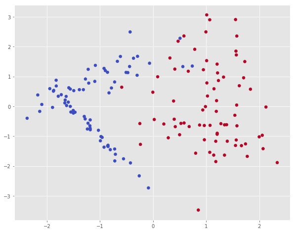
Now we will create our model using TensorFlow. I'm gonna explain some of the function in TensorFlow.
tf.random_normal- Generate Random number from Normal Distributiontf.matmul(A, B)- Multiply matrices A & B - A * Btf.sigmoid- Calculate Sigmoid Functiontf.reduce_mean- Equivalent tonp.meantf.train.GradientDescentOptimizer- Initialize Gradient Descent Optimizer Object
# Define Placeholders for X and Y
# None represents the number of training examples.
X = tf.placeholder(tf.float32, shape=[None, 2])
Y = tf.placeholder(tf.float32, shape=[None, 1])

# Weights and Biases
W = tf.Variable(tf.random_normal([2, 1]), name='weight')
b = tf.Variable(tf.random_normal([1]), name='bias')

# Hyposthesis
hypothesis = tf.sigmoid(tf.matmul(X, W) + b)

# Cost Function
cost = -tf.reduce_mean(Y * tf.log(hypothesis) + (1 - Y) *
                       tf.log(1 - hypothesis))

# Optimize Cost Function using Gradient Descent
train = tf.train.GradientDescentOptimizer(learning_rate=0.01).minimize(cost)

# Prediction and Accuracy
predicted = tf.cast(hypothesis > 0.5, dtype=tf.float32)
accuracy = tf.reduce_mean(tf.cast(tf.equal(predicted, Y), dtype=tf.float32))

# Start Session
sess = tf.Session()

# Initialize Variables
sess.run(tf.global_variables_initializer())

# Train the model
for step in range(10001):
    cost_val, _ = sess.run([cost, train], feed_dict={X: x, Y: y})
    if step % 1000 == 0:
    	# Print Cost Function
        print(step, cost_val)

# Accuracy report
h, c, a = sess.run([hypothesis, predicted, accuracy],
                       feed_dict={X: x, Y: y})
print("\nAccuracy: ", a)

# Plot decision boundary
plot_decision_boundary(lambda x: sess.run(predicted, feed_dict={X:x}), x)
0 0.402723
1000 0.188334
2000 0.161659
3000 0.151207
4000 0.145771
5000 0.142535
6000 0.140447
7000 0.139026
8000 0.138023
9000 0.137293
10000 0.13675
Accuracy: 0.946667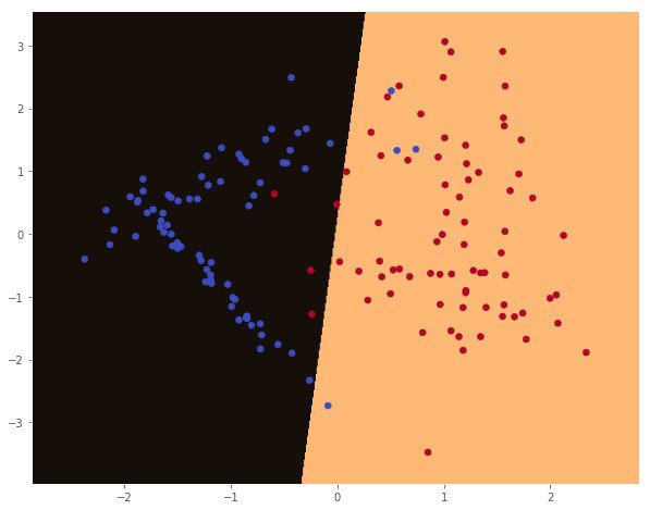
That's our Logistic Regression Model using TensorFlow. Hope this helps. Let me know if you found any errors.
Checkout this Github Repo for all the codes.
More Resources
Books
- Hand-On Machine Learning with Scikit-Learn and TensorFlow
- Learning TensorFlow
- TensorFlow for Deep Learning: From Linear Regression to Reinforcement Learning
Other Links
- Getting Started with TensorFlow - TensorFlow Official Website
- TensorFlow Tutorial For Beginners - Datacamp Community
- TensorFlow Tutorial - Edureka
- TensorFlow Tutorial: 10 minutes Practical TensorFlow lesson for quick learners